Configuration

This section describes how a simulation is configured using information read from files and command-line options. For an overview of how a simulation is performed and what parameters it requires see the User’s Guide. Configuration options specify the instrument, atmosphere and source to simulate, and how the simulation should be performed.

This package originated as a DESI-specific simulation tool but, as of v0.3, has no code dependencies on DESI software and makes no hardcoded assumptions that are specific to DESI. Instead, any fiber spectrograph and observing conditions can be configured. Several configurations are included with the code distribution (under specsim/data/config/) and described below. New configurations are straightforward to create using these examples as templates.

This document provides a user-oriented view of configuration, and focuses on the tasks of interpreting end editing configuration files. For a developer-oriented view, see the API documentation.

Configuration File

The top-level configuration is specified by a single YAML file with four main sections: atmosphere, instrument, source, and simulator. This top-level file refers to additional files containing tabulated data, which are generally large and packaged separately. For example, the DESI configuration refers to files in the desimodel package.

Most of the configuration is used to initialize the independent models of the atmosphere, instrument and source that come together in the simulator. However, there are also a few global configuration options that you should be familiar with:

name: DESI QuickSim

# Be verbose during the simulation?
verbose: no

# The base path is pre-pended to all non-absolute path values below.
# {...} will be expanded using environment variables.
base_path: '{DESIMODEL}/data'

# Specify the wavelength grid to use for simulation.
wavelength_grid:
    unit: Angstrom
    min: 3500.3
    max: 9999.7
    step: 0.1

The first two parameters are self explanatory. The base_path option establishes the link between a configuration file and a directory tree containing the tabulated data that it refers to. The wavelength_grid options specify the equally spaced wavelength grid used internally by the simulation, which should be chosen to cover the instrument throughput and should sample the instrument’s wavelength resolution sufficiently for a binned model of resolution effects. This wavelength grid is downsampled to the simulation output grid according to the simulator.downsampling parameter.

A valid configuration file is a YAML file whose hierarchy is specified using only mappings (dictionaries), with no sequences (lists). All mapping keys must be valid python identifiers, and custom objects are not supported.

The various configuration sections share some common syntax for specifying physical constants and tabular data, as described in the following sections.

Constants

Physical constants are grouped within a constants node and consists of a list of name-value pairs, for example:

constants:
    read_noise: 2.9 electron
    dark_current: 2.0 electron/(hour pixel**2)
    gain: 1.0 electron/adu

Units are required, except for dimensionless quantities, and must be separated from the value with some white space. Units are interpreted by the astropy.units module. Note that pixel is interpreted as a linear unit in this package, so that dark current is expressed in units of pixel**2.

Tabulated Data

Tabulated data is read using astropy.table.Table.read() so is very flexible. A simple table node to specify a function of wavelength might look like:

table:
    path: throughput.csv
    columns:
        wavelength: { index: 0, unit: Angstrom }
        throughput: { index: 1 }

In this example, the file format is automatically determined by the filename extension and the required columns are identified by their indices (0, 1) in the file. Tabulated data generally requires units, but these can be specified in the configuration file instead of the data file, for more flexibility.

Here is a more complex example of reading data from a binary table within a multi-HDU FITS file:

table:
    path: throughput.fits
    hdu: THRU
    wavelength: { name: wave }
    throughput: { name: thru }

In this case the HDU and columns are identified by their names in the FITS file.

Finally, some tabulated data uses different files to represent different options. For example, sky surface brightness tables under different conditions are specified by replacing the path node with a paths node as follows:

paths:
    dark: dark-sky.csv
    grey: grey-sky.csv
    bright: bright-sky.csv

For additional examples of specifying tabular data, refer to the configurations included with this package and described below.

DESI Configuration

The DESI configuration refers to data files maintained in the desimodel package, which the user must separately install. The linkage is established via the DESIMODEL environment variable via the following line in desi.yaml:

base_path: '{DESIMODEL}/data'

The DESI configuration reads tabulated data files directly from desimodel so any changes there propagate automatically to the simulation. Note, however, that the specsim DESI configuration does not read constants directly from desimodel/desi.yaml. Instead, the following values are copied from that file into this package’s DESI configuration file (also called desi.yaml), in order to achieve a unified and consistent configuration scheme:

desimodel name	specsim name
area.M1_diameter	instrument.constants.primary_mirror_diameter
fibers.diameter_um	instrument.constants.fiber_diameter
area.obscuration_diameter	instrument.constants.obscuration_diameter
area.M2_support_width	instrument.constants.support_width
ccd.*.readnoise	instrument.cameras.*.constants.read_noise
ccd.*.darkcurrent	instrument.cameras.*.constants.dark_current
ccd.*.gain	instrument.cameras.*.constants.gain
exptime	observation.constants.exposure_time

In addition to name mappings above, the specsim configuration values all have machine-readable units attached in a constants section (unlike the corresponding desimodel values, where units are specified in comments).

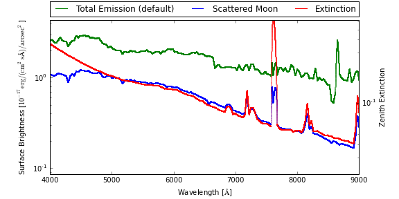
Atmosphere

The following plot summarizes the default DESI atmosphere used for simulations, and was created using:

config = specsim.config.load_config('desi')
specsim.atmosphere.initialize(config).plot()

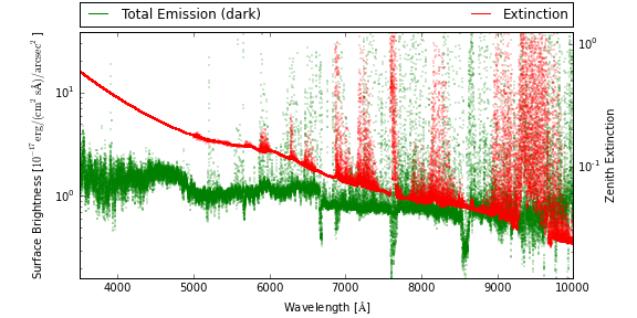
The default atmosphere has the moon below the horizon. To simulate grey or bright conditions, add scattered moon light by modifying the relevant parameters in the configuration, or else by changing attributes of the initialized atmosphere model. For example:

atm = specsim.atmosphere.initialize(config)
atm.airmass = 1.3
atm.moon.moon_zenith = 60 * u.deg
atm.moon.separation_angle = 50 * u.deg
atm.moon.moon_phase = 0.25
atm.plot()

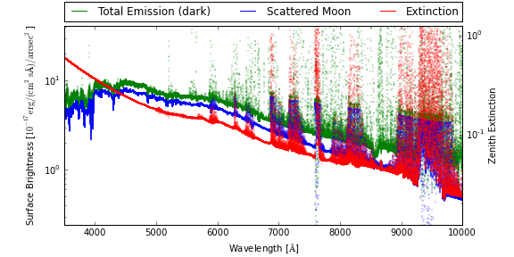
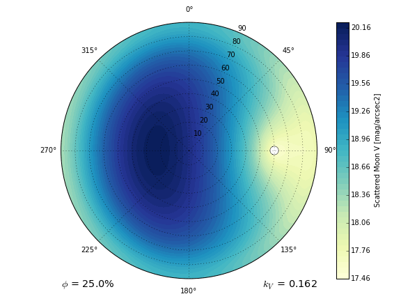
Note how total sky emission has increased significantly and is dominated by scattered moon at the blue end. To explore the dependence of the scattered moon brightness on the observed field, use specsim.atmosphere.plot_lunar_brightness(). For example:

specsim.atmosphere.plot_lunar_brightness(
    moon_zenith=60*u.deg, moon_azimuth=90*u.deg, moon_phase=0.25)

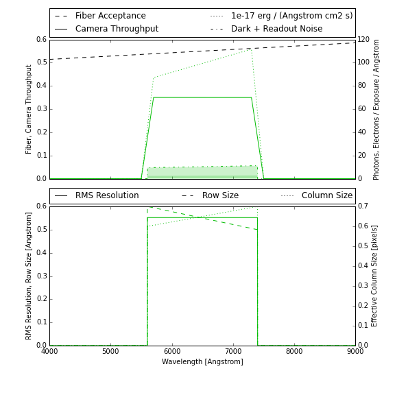
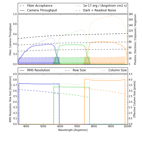
Instrument

The following plot summarizes the default DESI instrument configuration, and was created using:

config = specsim.config.load_config('desi')
specsim.instrument.initialize(config).plot()

Test Configuration

The test configuration is intended for self-contained tests and demonstrations of this packages capabilities and only refers to small tabulated data files that are distributed with this package. As a result, the test configuration is deliberately over-simplified and should only be used for testing purposes.

Atmosphere

The following plot summarizes the default test atmosphere used for simulations, and was created using:

config = specsim.config.load_config('test')
specsim.atmosphere.initialize(config).plot()

Note that the test atmosphere has the moon above the horizon by default.

Instrument

The following plot summarizes the default test instrument configuration, and was created using:

config = specsim.config.load_config('test')
specsim.instrument.initialize(config).plot()