User’s Guide
SpecSim is a python package for quick simulations of multi-fiber spectrograph response. For a quick introduction, browse the examples notebook or try one of the command-line programs.
A simulation has the following main components, as illustrated in the figure below:
An astrophysical source.
A model of the sky and atmosphere.
An instrument, consisting of a telescope and one or more cameras.
An observation is specified by:
An exposure time \(\Delta t\).
An observing airmass \(X\).
The table below lists all of the simulation modeling parameters described in this guide, and specifies their units and which component they are associated with.
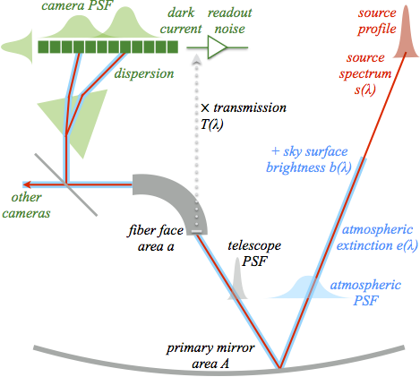
Overview of the simulation components and parameters. Camera components are shown in green, telescope components in gray, sky / atmospheric components in light blue, and source components in red.
Source Model
An astrophysical source is represented by its spectral energy distribution (SED) \(s(\lambda)\) and its profile. We assume that a source’s profile is independent of its SED.
Atmosphere Model
The atmosphere adds its own emission spectrum \(b(\lambda)\) to that of the source and then both are attenuated by their passage through the atmosphere by the extinction factor:
where \(X\) is the airmass of the observation. The atmosphere model also specifies a point-spread function (PSF).
Instrument Model
The instrument consists of a telescope and one or more cameras. The telescope is described by the unobscured collecting area of its primary mirror \(A\), used to normalize the source and sky fluxes, and the input face area \(a\) of its individual fibers, used to normalize the sky flux. The telescope also has an optical PSF that is convolved with the atmospheric PSF and the source profile to determine the profile of light incident upon the fiber entrance face in the focal plane. The overlap between this convolved profile and the fiber aperture determines the fiber acceptance fraction \(f_S(\lambda)\) (see Fiber Acceptance Fraction Calculations for details). The resulting flux \(F(\lambda)\) in erg/\(\text{\AA}\) entering the fiber is:
where \(\Delta t\) is the exposure time.
All calculations are performed on a fine wavelength grid \(\lambda_j\) that covers the response of all cameras with a spacing that is smaller than the wavelength extent of a single pixel by at least a factor of five. The number of photons entering the fiber with wavelengths \(\lambda_j \le \lambda < \lambda_{j+1}\) is then given by:
with wavelength bin widths and centers:
The remaining calculations are performed separately for each camera, indexed by \(i\). The throughput function \(T_i(\lambda)\) gives the combined wavelength-dependent probability that a photon incident on a fiber results in an electron detected in the camera’s CCD.
The distribution of detected electrons over sensor pixels is determined by the camera’s dispersion function \(d_i(\lambda)\) and effective wavelength resolution \(\sigma_i(\lambda)\). We first apply resolution effects using a convolution matrix \(R_{jk}\), resulting in:
electrons detected in camera \(j\) and associated with the detected wavelength \(\overline{\lambda}_k\). Next, the continuous pixel coordinate (in the wavelength direction) associated with the detected wavelength is calculated as \(d(\overline{\lambda}_k)\) and used to re-bin electron counts from the fine detected wavelength grid \(N^{eh}_{ik}\) to sensor pixels \(N^{eh}_{ip}\).
Finally, the sensor electronics response is characterized by a gain \(G_i\), dark current \(I_{dk}\) and readout noise \(\sigma_{ro,i}\). The resulting signal in detected electrons is given by:
with a corresponding variance:
where \(n_{ip}\) is the effective trace width in pixels for wavelength pixel \(p\), and we assume that read noise is uncorrelated between pixels (so its variance scales with \(n_{ip}\)).
Parameter |
Component |
Description |
|---|---|---|
\(\Delta t\) |
Instrument |
Exposure time |
\(X\) |
Atmosphere |
Observing airmass |
\(\lambda_i\) |
Configuration |
Fine wavelength grid |
\(s(\lambda)\) |
Source |
Source SED |
\(b(\lambda)\) |
Atmosphere |
Sky surface brightness |
\(e(\lambda)\) |
Atmosphere |
Atmospheric extinction |
\(A\) |
Instrument |
Primary unobscured area |
\(a\) |
Instrument |
Fiber entrance area |
\(f_S(\lambda)\) |
Source+Instrument |
Fiberloss fraction |
\(T_i(\lambda)\) |
Camera |
Transmission throughput |
\(d_i(\lambda)\) |
Camera |
CCD row size |
\(\sigma_i(\lambda)\) |
Camera |
CCD resolution |
\(n_{ip}\) |
Camera |
CCD trace width |
\(I_{dk,i}\) |
Camera |
Sensor dark current |
\(G_i\) |
Camera |
Readout gain |
\(\sigma_{ro,i}\) |
Camera |
Readout noise |